Capsule Networks against Medical Imaging Data Challenges — in Julia
A native Julia/Flux.jl reproduction of the LABELS@MICCAI 2018 study by Jiménez-Sánchez, Albarqouni & Mateus — capsule networks vs. CNNs under the data constraints that define medical imaging: scarce annotations, imbalanced classes, and the question of whether augmentation helps.
Background
Sabour, Frosst & Hinton's capsule networks (NeurIPS 2017) replace scalar neurons with small vectors — capsules — whose length encodes the probability that an entity exists and whose orientation encodes the entity's pose: position, scale, stroke thickness, skew. Instead of max-pooling away spatial relationships, a capsule layer routes by agreement: a lower capsule sends its output to the higher capsule whose prediction it agrees with, so part–whole relationships are negotiated rather than discarded.
That design promises something specifically valuable for medical imaging: less appetite for data. If equivariance is built in, the network shouldn't need thousands of augmented examples to learn that a rotated lesion is still a lesion. Jiménez-Sánchez, Albarqouni & Mateus put this claim to the test at LABELS@MICCAI 2018, comparing CapsNet against LeNet and against the deliberately-strong CNN baseline from the original capsule paper, on four datasets (MNIST, Fashion-MNIST, TUPAC16 mitosis detection, DIARETDB1 diabetic retinopathy) under three controlled stressors:
Limited data — train on stratified fractions of the training set;
Class imbalance — starve selected classes to 20% of their examples;
Data augmentation — small rotations (and flips where they make sense) appended to the training set.
Their finding: capsule networks degrade more gracefully than both CNNs as data shrinks or skews. This project reproduces that entire experimental apparatus in Julia.
The architecture
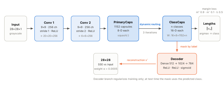
Figure 1. The reproduced CapsNet. Two 9×9 convolutions produce a 6×6×256 tensor read as 1152 primary capsules of 8 dimensions; three iterations of routing-by-agreement produce one 16-D capsule per class. Capsule length is the class score. During training the winning capsule (masked by the true label) is decoded back to 784 pixels, and the reconstruction error regularizes the encoder — at test time the mask uses the predicted label instead.
A capsule's activation is kept in the unit ball by the squash nonlinearity, which preserves orientation while mapping length to \([0,1)\):
\[ \mathbf{v}_j \;=\; \frac{\lVert \mathbf{s}_j \rVert^2}{1+\lVert \mathbf{s}_j \rVert^2}\,\frac{\mathbf{s}_j}{\lVert \mathbf{s}_j \rVert} \]Each primary capsule \(i\) predicts every class capsule \(j\) through a learned transform, \(\hat{\mathbf{u}}_{j|i} = \mathbf{W}_{ij}\,\mathbf{u}_i\), and routing-by-agreement decides how much each prediction counts. With logits \(b_{ij}\) initialized to zero, three iterations of:
\[ c_{ij} = \operatorname{softmax}_j(b_{ij}), \qquad \mathbf{s}_j = \sum_i c_{ij}\,\hat{\mathbf{u}}_{j|i}, \qquad \mathbf{v}_j = \operatorname{squash}(\mathbf{s}_j), \qquad b_{ij} \mathrel{+}= \hat{\mathbf{u}}_{j|i}\cdot\mathbf{v}_j \]Classification is trained with the margin loss, summed over classes and averaged over the batch (\(T_k = 1\) for the true class):
\[ L_k = T_k\,\max(0,\, m^+ - \lVert \mathbf{v}_k \rVert)^2 \;+\; \lambda\,(1-T_k)\,\max(0,\, \lVert \mathbf{v}_k \rVert - m^-)^2 \]with \(m^+{=}\,0.9\), \(m^-{=}\,0.1\), \(\lambda{=}\,0.5\), plus a reconstruction term weighted by \(\alpha = 5\times10^{-4}\) so it regularizes without dominating:
\[ \mathcal{L} \;=\; \sum_k L_k \;+\; \alpha \,\lVert \hat{\mathbf{x}} - \mathbf{x} \rVert^2 \]Every number in the port is normative — copied from the reference and asserted where a test can reach it:
| Component | Value (identical to reference) |
|---|---|
| Conv 1 / Conv 2 | 256 filters, 9×9, valid, ReLU; stride 1 then stride 2 |
| Primary capsules | 1152 capsules × 8-D (= 6·6·32 maps), squash |
| Class capsules | \(n\) × 16-D, transform \(\mathbf{W} \in \mathbb{R}^{16\times8\times1152\times n}\) |
| Routing | 3 iterations, softmax over classes |
| Decoder | Dense 16·\(n\) → 512 → 1024 → 784, ReLU/ReLU/sigmoid |
| Loss | margin (\(0.9/0.1/0.5\)) + \(5{\times}10^{-4}\) · reconstruction SSE |
| Optimizer | Adam, lr \(10^{-3}\), ×0.95 exponential decay per epoch |
| Batch size | 64 (CapsNet), 128 (CNNs) |
The two comparison networks
LeNet — the classic: zero-pad to 32×32, two conv+maxpool stages (6 then 16 filters at 5×5), then dense 120 → 84 → \(n\). Exactly 61,706 trainable parameters at \(n{=}10\); the test suite asserts that count.
Baseline CNN — the deliberately strong baseline from the capsule paper: three 5×5 convolutions at 256/256/128 channels, "dense" layers expressed as 16×16 and 1×1 convolutions (328 and 192 channels), dropout 0.5, and L2 weight decay \(5\times10^{-4}\). At roughly 25M parameters it out-muscles CapsNet's ~8.2M — which is what makes CapsNet's low-data behavior interesting rather than a parameter-count artifact.
The three data challenges
The experiment harness stresses training data three ways, each a pure function LabeledData → LabeledData with an explicit RNG:
# 1. Limited data — stratified: keep pct% of every class
train = limit_data(train, 10; rng)              # 10% of MNIST ≈ 6,000 images

# 2. Class imbalance — starve selected classes to pct% (digits 0 and 8 → labels 1 and 9)
train = unbalance_data(train, [1, 9], 20; rng)

# 3. Augmentation — append ±10° rotations of 5% of samples (+ flips for Fashion)
train = augment_data(train; flips=false, rng)
These mirror the reference's percentage_train, unbalance_dict, and augment switches exactly — including details that are easy to get subtly wrong, like stratifying the limited-data subsample per class and appending (not replacing with) the augmented copies.
The port
MedCapsNet is a self-contained Julia package (Julia ≥ 1.10, Flux 0.16):
| Layer | Files | What it holds |
|---|---|---|
| Capsule math | src/layers.jl | squash, safe_norm, primary_capsules, prediction_vectors, routing |
| Models | src/capsnet.jl, src/baselines.jl | CapsNet, lenet, baseline_cnn |
| Losses | src/losses.jl | margin_loss, reconstruction_loss, capsnet_loss, cnn_loss |
| Data | src/data.jl | loaders, the three challenge transforms, medical JLD2 I/O, Macenko |
| Training | src/train.jl | generic train! — Adam + decay, best-validation checkpointing |
| Evaluation | src/metrics.jl | batched prediction, confusion matrix, per-class P/R/F1 |
| Figures | src/visualize.jl | reconstruction grids, capsule-perturbation grids |
| Entry points | scripts/ | train.jl, test.jl, visualize.jl, run_experiments.jl, two preprocessors |
Two implementation choices worth calling out for anyone porting TensorFlow capsule code to Julia:
Channel grouping across memory layouts. The reference reshapes its (B, 6, 6, 256) row-major tensor to (B, 1152, 8), which silently groups 8 consecutive channels at one spatial position into each capsule. Julia is column-major with WHCN layout, so the equivalent is not a bare reshape — it's reshape(permutedims(h, (3,1,2,4)), 8, 1152, B). A wrong permutation here still produces the right shapes, still trains, and still squashes to valid norms; only the capsule semantics quietly change. The review process hand-verified the index algebra rather than trusting shape-level tests.
Routing that survives automatic differentiation. Zygote (Flux's AD) rejects array mutation, so the routing loop is written with rebinding (b = b .+ agreement) and the logits are initialized with an AD-safe zero(T) .* sum(û; dims=1) rather than a zeros(...) literal — which also keeps the code generic over array types. The unrolled 3-iteration loop is differentiated end-to-end, exactly like the reference's static TF graph.
How it was built
The port was executed as 18 test-driven tasks, each implemented by a fresh agent against a written brief, each independently reviewed for spec compliance and code quality before the next began, with a final whole-branch review at the end. The suite grew task by task to 64 assertions — not just shape checks: hand-computed margin-loss values, a routing property test (capsules voting coherently for a class must out-length incoherent votes), a train-checkpoint-reload round-trip that must reproduce the best validation loss bit-for-bit, and a synthetic H&E image that must separate hematoxylin from eosin.
What reimplementation found
Reproducing a paper's code is a form of review, and this one surfaced real findings — all in the plan for the port rather than in the reference:
A stain-separation bug the tests caught. The port replaces Vahadane stain normalization with Macenko (SVD on optical densities — no sparse-NMF library exists in Julia). The first-draft Macenko picked the hematoxylin stain vector as the one with the larger blue optical-density component — intuitive ("hematoxylin is the blue stain") and wrong. Hematoxylin looks blue-purple because it absorbs red; on unit-normalized OD directions the blue component comparison actually inverts, selecting eosin. The synthetic-image test failed, the fix (compare the red OD component, as standard Macenko implementations do) was derived from the failure, and the reviewer independently re-derived the optics before it merged. A shape-level test would never have caught this.
A flaky test traced to an unseeded initializer. A "does the trainer learn?" test failed roughly one run in three: the toy model's Dense layer drew its weights from the global RNG while everything else was seeded. Seeding the initializer made the suite deterministic — and revealed that ~25% of seeds genuinely fail a "5 epochs is enough to learn" assertion on a 64-sample toy problem. Reproducibility bugs hide easily behind assertions that are merely usually true.
Assorted spec-level defects — a CSV format whose imbalance label ("1,9@20") embedded a comma into a comma-separated file, an include order that couldn't compile because a method's type annotation resolved before the type existed, dependency compat pins that silently raised the Julia floor above the advertised one. Each was caught by a reviewer or a failing build, not by luck.
Results
The low-data regime is where the paper's claim lives, so that is what the reproduction sweeps: both architectures trained on 1%, 5%, and 10% of MNIST (10 epochs, Adam 10⁻³ with ×0.95/epoch decay, best-validation checkpoint, seed 1), evaluated on the untouched 10,000-image test set. LeNet additionally gets the full-data, imbalance, and augmentation configurations — it is cheap enough on CPU.
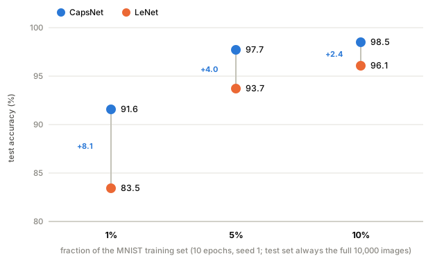
Figure 2. Test accuracy in the low-data regime (10 epochs, seed 1). CapsNet's advantage is largest exactly where the paper predicts: +8.1 points at 1% of the training data (550 images), narrowing to +2.4 points at 10% — built-in equivariance pays most when examples are scarcest. LeNet reaches 98.75% with the full training set (table below); the CapsNet configurations were trained on CPU (see the GPU postscript).
| Configuration | Training images | CapsNet | LeNet |
|---|---|---|---|
| 1% of MNIST | 550 | 91.55% | 83.45% |
| 5% of MNIST | 2,750 | 97.70% | 93.70% |
| 10% of MNIST | 5,501 | 98.51% | 96.07% |
| 100% of MNIST | 55,000 | — | 98.75% |
| Imbalance (digits 0, 8 → 20%) | 46,364 | — | 98.73% (starved-class recall 0.986 / 0.971) |
| Augmented (+5% rotated copies) | 57,750 | — | 98.92% |
The dashes are honest budget lines, not gaps in the port: a full-data CapsNet run is ~10× the 10% cost, and the imbalance/augmentation configurations train on near-full data — the CLI runs them with one flag each (--unbalance 1,9@20, --augment), and the full three-seed sweep command is in the reproduction section.
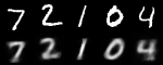
Figure 3. Inputs (top) and decoder reconstructions from the winning 16-D class capsule (bottom), CapsNet trained on 10% of MNIST. The decoder sees only 16 numbers per image — the blur is the price of that bottleneck, and the point: the capsule keeps what identifies the digit.
Perturbing one dimension of the winning capsule and decoding each variant shows what the 16 dimensions learned to encode — stroke thickness, slant, width — without ever being told to:
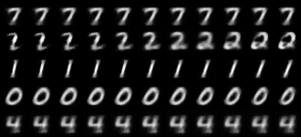
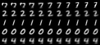
Figure 4. Capsule-dimension perturbations: each row is one test digit, each column decodes the winning capsule with one dimension shifted through [−0.5, 0.5] in 11 steps (center column = unperturbed). Two of the sixteen dimensions shown: the first (dim 8) morphs stroke topology — watch the 2's loop open and close — while the second (dim 5) shifts stroke weight and the 7's serif. Nobody labeled these factors; routing discovered them.
Against the paper's own numbers
The reference study trained 432 networks — 3 architectures × 9 data conditions × 4 repetitions × 4 datasets, 50 epochs with early stopping — and reports mean F1-scores (Table 2 of arXiv:1807.07559). This page's runs are a far smaller budget, so the honest comparison is of trends, not cells:
| MNIST fraction | LeNet — paper (F1) | CapsNet — paper (F1) | LeNet — this port (acc.) | CapsNet — this port (acc.) |
|---|---|---|---|---|
| 1% | 0.909 | 0.943 | 83.45% | 91.55% |
| 5% | 0.961 | 0.975 | 93.70% | 97.70% |
| 10% | 0.975 | 0.985 | 96.07% | 98.51% |
Paper columns: mean F1 over 4 repetitions, 50 epochs with early stopping, from the original TensorFlow implementation — not outputs of this port. Port columns: test accuracy, seed 1, 10 epochs, from the Julia code. Different metric and training budget; the cells are not directly comparable, the trend is.
Both halves tell the same story: CapsNet leads at every fraction and the lead is largest where data is scarcest — the paper's gap shrinks from +3.4 F1 points at 1% to +1.0 at 10%, the port's from +8.1 accuracy points to +2.4. The port's wider gaps are consistent with its shorter budget. On the medical datasets, the paper reports the same graceful degradation (on DIARETDB1 CapsNet beats both CNNs at every fraction; on TUPAC16 it trails LeNet at 1% and leads from 10% up) — the yardstick the medical pipelines here will be measured against once the registration-gated data lands.
The medical pipelines
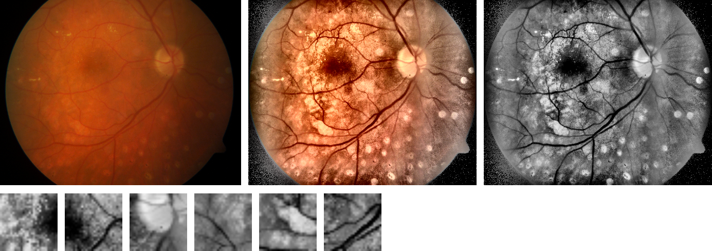
Figure 5. The retinopathy preprocessing pipeline, run by this package's own code on a real fundus photograph (DIARETDB0, the sister dataset — see the data-access note below): original → border-cropped + contrast-enhanced (CLAHE-equivalent) → green channel, then 28×28 patches extracted at lesion centers-of-mass — the exact input format the capsule network trains on.
Both medical datasets from the study are supported end-to-end — and the difficulty of even obtaining them today is the paper's thesis writing itself: the original DIARETDB1 host (a 2007-era university server) is offline, the one public mirror labeled "DIARETDB1" actually contains its predecessor DIARETDB0, and TUPAC16 sits behind challenge registration. Figure 5 therefore demonstrates the pipeline on a DIARETDB0 image (same camera, same 50° protocol, coarser labels); the per-lesion training protocol below runs unchanged the moment the real DIARETDB1 lands in raw_data/ (a Kaggle mirror exists for account holders). The pipelines themselves are validated with synthetic fixtures and unit tests:
TUPAC16 (mitosis detection, 2 classes). High-power-field histology tiles are stain-normalized with Macenko, the hematoxylin concentration channel is extracted, and 100×100 patches are cut around annotated mitosis centers (30 jittered positives per image; 3 negatives from mitosis-free grid cells), resized to 28×28. This is the port's one documented algorithmic deviation: the reference uses Vahadane normalization via the SPAMS library, which has no Julia equivalent; Macenko is the standard substitute.
DIARETDB1 (diabetic retinopathy, 2 classes). Fundus images are cropped of their black border, contrast-enhanced (CLAHE-equivalent adaptive equalization), reduced to the green channel, and 200×200 patches are extracted at lesion centers-of-mass on a 300-px grid — exudates (soft+hard) vs. hemorrhages+red small dots — resized to 28×28.
Both write the same data.jld2 contract the trainer consumes (train/val/test arrays plus the training mean), so a medical run is just:
julia --project=. scripts/preprocess_diaretdb1.jl
julia --project=. scripts/train.jl medical capsnet --datadir data/diaretdb1
julia --project=. scripts/test.jl  medical capsnet --datadir data/diaretdb1
Postscript: porting the training loop to Apple-GPU (Metal)
The package now supports --device gpu on Apple Silicon via Metal.jl — and getting there was its own small research story, told here because the negative results are as instructive as the wins:
The naive port lost to the CPU. With the capsule layer written as a materialized broadcast (the straightforward translation of the reference TF code), a batch-64 gradient step took 2,840 ms on the GPU vs 1,425 ms on CPU — the backward pass through a 380 MB temporary is kernel-launch soup.
Reformulating prediction as batched matrix multiplication fixed the math path.
û_{j|i} = W_{ij} u_iover 1,152 capsules is exactly a batched matmul; expressed that way (hitting Apple's MPS on GPU, BLAS on CPU) the CPU step dropped ~40% and the GPU pulled ahead of the CPU per-step — verified across five independent benchmark runs.Then the OS killed the training run. Multi-epoch GPU training ballooned to 62.8 GB of unified memory on a 24 GB machine before macOS's jetsam killed it. Half the cause is a known ecosystem trap — Julia's GC never feels GPU buffer pressure, fixed here with a periodic reclaim hook in the trainer. The other half, isolated by bisection (each layer run alone with memory sampling), is a genuine buffer leak inside Metal.jl's MPS
matmul!— the exact op the speedup relies on — which no amount of GC can reclaim.
Where that leaves things: LeNet and the Baseline CNN train fully on the GPU (10 epochs, 1.75 GB peak, verified bounded), and the LeNet results above were produced that way; CapsNet training stays on CPU until the upstream leak is fixed, which the batched-matmul reformulation made perfectly practical (~15 minutes for the 10%-data model on this page). Every measurement, the bisection procedure, and the per-op memory timelines are in the repository's benchmark script and README.
Reproduce everything
git clone https://github.com/BhavyaQuantDeveloper/MedCapsNet && cd MedCapsNet
julia --project=. -e 'using Pkg; Pkg.instantiate(); Pkg.test()'   # 72/72

# the figures on this page
julia --project=. scripts/train.jl mnist capsnet --epochs 10 --percentage 10 --seed 1 --modeldir models/page/capsnet-p10
julia --project=. scripts/test.jl  mnist capsnet --modeldir models/page/capsnet-p10
julia --project=. scripts/visualize.jl mnist --modeldir models/page/capsnet-p10

# the full experiment sweep from the paper (days of compute; --device gpu helps only marginally — see README)
julia --project=. scripts/run_experiments.jl mnist --epochs 25 --seeds 1,2,3
Honest limitations. These are single-seed, 10-epoch runs (CapsNet on CPU, LeNet on GPU) on MNIST — a demonstration that the reproduced pipeline behaves like the paper's, not a re-derivation of its tables (the reference trains far longer, averages seeds, and spans four datasets). The full-fidelity sweep is one command above; the medical datasets additionally need registration-gated downloads. Beyond the Macenko substitution, two reference behaviors are approximated and flagged in the README: the CLAHE parameterization, and the trainer's exponential-decay rate, which the reference leaves unspecified.
References
A. Jiménez-Sánchez, S. Albarqouni, D. Mateus. Capsule Networks against Medical Imaging Data Challenges. LABELS@MICCAI 2018. arXiv:1807.07559
S. Sabour, N. Frosst, G. E. Hinton. Dynamic Routing Between Capsules. NeurIPS 2017. arXiv:1710.09829
M. Macenko et al. A method for normalizing histology slides for quantitative analysis. ISBI 2009.
Reference implementation: ameliajimenez/capsule-networks-medical-data-challenges (TensorFlow 1.4, builds on @ageron's CapsNet).
This port: BhavyaQuantDeveloper/MedCapsNet (Julia ≥ 1.10, Flux 0.16).